Taking Eclipse Qrisp for a spin
Looking around at many of the dominant libraries used for coding quantum algorithms today (IBM Qiskit, Google Cirq, Amazon BraKet, and so on), it’s hard to believe we will be using any of these libraries in 10 years time. It’s not that any of these libraries are bad, it’s just that it’s terribly inconvenient for end users to have to rewrite their client code whenever they want to try out their code on a different platform. There is clearly a need to adopt a common standard for writing quantum client code.
This brings me to the subject of today’s blog, the open-source Eclipse Qrisp client library (sponsored by the Fraunhofer Institute), which I believe has a fair chance of winning the race to become the quantum client library of the future. Let me explain why I think so.
In my view, the following are the minimum prerequisites for a client library to achieve widespread adoption:
-
Must be open source: this is already true for the vast majority of client libraries currently on offer, with some exceptions.
-
Should probably be non-commercial: when it comes to the currently available commercial libraries, existing companies are pursuing their own commercial imperatives. It seems more likely that a common standard will emerge from the non-profit sector (third-level, government-sponsored, and so on).
-
Must incorporate high-level programming concepts: current quantum libraries have often been compared to assembly language programming. In fact, considering that quantum gates are analogous to Boolean gates, the current programming paradigm is actually closer to the level of designing chip circuits.
-
Must be written in Python: there have been numerous attempts to establish client libraries written in languages other than Python. I believe these experiments are doomed to fail, as Python is already firmly established as the language of scientific computing.
-
Must integrate elegantly with Python syntax: this is a bit of a challenge, because quantum computing has oddities that are difficult to capture in conventional computing syntax.
First of all, Qrisp is a good candidate for a client library because it satisfies these basic criteria. But that’s not all.
Thanks to some well-considered architectural decisions, Qrisp integrates exeptionally cleanly with Python syntax, enabling a compact and elegant coding style. The creators of Qrisp have also invested a lot of time and effort in their implementation of basic arithmetical algorithms, exploiting the fruits of the latest research and publishing a string of original papers in this field. As a result, algorithms written with the Qrisp library are highly performant when compared with other quantum libraries.
First example
To illustrate the capabilities of the Qrisp library, we present an
example that uses Grover’s algorithm to solve the prime factorization
problem. That is, given an integer r equal to the product of two
primes, p and q (so that r=pq), we will find the prime factors p
and q. Given an integer r = p * q (where p and q are prime), we
use Grover’s algorithm to find the prime factors (p, q).
To solve the factorization problem:
-
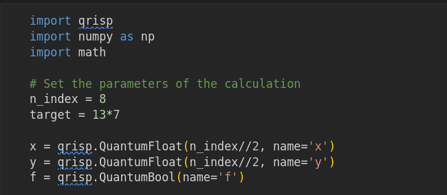
We define two integer registers
xandy(of typeQuantumFloatwith zero exponent). -
We define the oracle function as
f(x,y) = (x*y == target), wheretargetis the value we are trying to factorize. -
We proceed by initializing the quantum state in a superposition of every possible combination of factors
xandy, and then use the Grover search algorithm to find the values of(x,y)that satisfy the oracle condition,x*y==target.
import qrisp
import numpy as np
import math

# Set the parameters of the calculation
n_index = 8
target = 13*7

x = qrisp.QuantumFloat(n_index//2, name='x')
y = qrisp.QuantumFloat(n_index//2, name='y')
f = qrisp.QuantumBool(name='f')

def n_grover_iter(n_index_bits, target_set_size):
    # Calculate the required number of Grover iterations
    #   n_index_bits: number of bits used for the index
    #   target_set_size: number of states in the target (solution) set
    return math.ceil( (2**(n_index_bits/2))*np.pi/(4.0*np.sqrt(target_set_size)) - 0.5 )

def phase_oracle_init(p):
    qrisp.z(qrisp.h(p))

def apply_oracle_phase():
    product = x * y
    qrisp.mcx(product, f, ctrl_state=target)  # Tests: (product == target)
    product.uncompute()

# Prepare the quantum state in an equal-weighted superposition (Walsh-Hadamard transform)
qrisp.h(x)
qrisp.h(y)

# Perform the Grover iterations
with qrisp.conjugate(phase_oracle_init)(f):
    for i in range(n_grover_iter(n_index, 2)):
        # Apply first Grover reflection operator
        apply_oracle_phase()
        # Apply second Grover reflection operator
        qrisp.h(x)
        qrisp.h(y)
        qrisp.mcx(x[:] + y[:], f, ctrl_state=0)
        qrisp.h(y)
        qrisp.h(x)

# Evaluate the circuit and show the measurement results
print(qrisp.multi_measurement([x, y]))
If you are familiar with a quantum computing library, you can probably guess what most of the code is doing. But it’s worth highlighting a few points from the preceding example that illustrate some of Qrisp’s unique features:
-
Uncomputing the multiplication operation:
def apply_oracle_phase():
  product = x * y
  qrisp.mcx(product, f, ctrl_state=target)
  product.uncompute()
The line
product = x * yimplicitly adds the gates required for the multiplication algorithm and puts the result into a new auxilary register, which is referenced byproduct. At the end of the function, the multiplication algorithm is uncomputed using the syntaxproduct.uncompute(), thereby freeing up the auxilary register. -
Uncomputing the phase oracle bit:
with qrisp.conjugate(phase_oracle_init)(f):
  # lines of code...
A common pattern in quantum computing is where you execute one or more lines of code bracketed between a compute \(V\) operation and an uncompute \(V^\dagger\) operation. This pattern is neatly captured by the
with qrisp.conjugate(…)idiom. In this example, the compute operation initializes the phase oracle by mapping \(|0\rangle\mapsto (|0\rangle - |1\rangle)/\sqrt{2}\) (executed at the start of thewithblock) and then the uncompute operation resets the phase oracle back to \(|0\rangle\) (executed at the end of thewithblock). -
Evaluating the circuit and parsing the results:
print(qrisp.multi_measurement([x, y]))Remarkably, the Qrisp library enables you to specify the measured quantum registers, send the circuit to the built-in simulator, and then parse and print the results in just a single line of code!
-
Look, no circuit!
You might be wondering, what happened to the quantum circuit in this example? Well, the quantum circuit is still an important concept in Qrisp programming, but you do not need to access it all that often.
Where is the circuit?
You might be wondering where the quantum circuit comes into play, as it is not directly referenced anywhere in the preceding example.
Qrisp manages quantum circuits as follows:
Every quantum variable you instantiate in Qrisp is initially associated with its own circuit (quantum session). However, when you combine quantum variables in some non-trivial way (causing quantum entanglement), their associated circuits are automatically merged together.
This is surely the ideal solution for managing circuits: for almost every conceivable use case, this convention guarantees that your circuits will automatically have exactly the intended scope. Manual management of the association between circuits and quantum variables therefore becomes unnecessary.
Note that every circuit is wrapped in a qrisp.QuantumSession instance,
which is effectively an abstraction of the quantum circuit. Given any
quantum variable instance qv, you can access its quantum session as
qv.qs.
import qrisp

qv = qrisp.QuantumVariable(4, name='qv')
qrisp.x(qv)

qsession = qv.qs
print(qsession.statevector())
|1111>
Allocation and initialization
Upon instantiation, all qubits in a quantum variable are 0 by default (the default qubit state on quantum hardware). You can initialize a quantum variable to a non-zero value using the slice assignment operation:
# Allocation and initialization
from qrisp import QuantumFloat

qf = QuantumFloat(3, name='qf')    # 3-qubit integer

qf[:] = 5

print(qf)
WARNING:2025-11-20 13:07:52,079:jax._src.xla_bridge:909: An NVIDIA GPU may be present on this machine, but a CUDA-enabled jaxlib is not installed. Falling back to cpu.
{5: 1.0}
You can use the slice assignment syntax to assign a variable at most once (while the variable is ``fresh''). If you try to initialize a variable more than once, you get an error (which reflects the underlying reality of qubit registers, which can only be set to a specific value if you know what the preceding state was).
You can also initialize a quantum variable using an initializing dictionary, which represents a quantum superposition of states. An initializing dictionary is specified in the following format:
{value: complex_amplitude, value: complex_amplitude, ...}
Where the format of the value keys depends on the type of quantum
variable you are initializing, as shown in the following example:
# Allocation and initialization
import numpy
import qrisp
from qrisp import QuantumVariable, QuantumFloat, QuantumBool, QuantumChar, QuantumString

qv = QuantumVariable(3, name='qv')
qf = QuantumFloat(3, name='qf')
qb = QuantumBool(name='qb')
qc = QuantumChar(name='qc')
qs = QuantumString(size=7)

qv[:] = {'001': numpy.sqrt(0.5), '011': numpy.sqrt(0.5)}
qf[:] = {3: numpy.sqrt(2.0/3.0), 7: numpy.sqrt(1.0/3.0)}
qb[:] = True
qc[:] = {'a': 1, 'b': 1, 'c': 1}

print(qv)
print(qf)
print(qb)
print(qc)
{'001': 0.5, '011': 0.5}
{3: 0.66667, 7: 0.33333}
{True: 1.0}
{'a': 0.3333333333333333, 'b': 0.3333333333333333, 'c': 0.3333333333333333}
Note one potential point of confusion here: while the initializing dictionary specifies the weights as complex amplitudes, the dictionary output by the print command shows the weights as the square of the amplitude norm.
The amplitudes you supply to the initializing dictionary
do not need to be normalized. This can be convenient for initializing a
state to have alternative values of equal weight, as demonstrated for
the case of the quantum char in the preceding example,
qc[:] = {'a': 1, 'b': 1, 'c': 1}.
|
Gates
If you just want to apply quantum gates to quantum registers and qubits,
you have the standard repertoire of gates available, familiar from such
libraries as IBM Qiskit, Google cirq, Amazon braket, and so on. Create
some QuantumVariable instances and start applying gate operations in
the familiar way:
from qrisp import QuantumVariable, h, x, y, z, cx

qv1 = QuantumVariable(3)    # Creates a 3-qubit register
qv2 = QuantumVariable(3)    # Creates another 3-qubit register

h(qv1)          # Hadamard
y(qv2)          # Pauli Y
cx(qv1, qv2)    # CNOT

print(qv2.qs)
QuantumCircuit:
---------------
┌───┐
qv1.0: ┤ H ├──■────────────
├───┤ │
qv1.1: ┤ H ├──┼────■───────
├───┤ │ │
qv1.2: ┤ H ├──┼────┼────■──
├───┤┌─┴─┐ │ │
qv2.0: ┤ Y ├┤ X ├──┼────┼──
├───┤└───┘┌─┴─┐ │
qv2.1: ┤ Y ├─────┤ X ├──┼──
├───┤ └───┘┌─┴─┐
qv2.2: ┤ Y ├──────────┤ X ├
└───┘ └───┘
Live QuantumVariables:
----------------------
QuantumVariable qv1
QuantumVariable qv2
You have a few different options for selecting qubits from a register:
-
Apply the gate to every qubit in the register:
h(qv1) -
Apply the gate to just one qubit at a time:
h(qv1[2]) -
Apply the gate to a slice of qubits:
h(qv[0:2])
Though not supported by Qrisp, on my own personal feature wishlist, I’d like to see the ability to use a bitmask to select which qubits to affect — for example, something like:
qv8 = QuantumVariable(8, name='qv8')

h(qv8, '11100110')    # Apply h() only to the bits flagged with '1'
Basic arithmetic with QuantumFloat
You can also perform arithmetic operations using the QuantumFloat and
QuantumModulus types. Looking at the available quantum types in Qrisp,
I initially wondered why there wasn’t any quantum integer type. It turns
out that integers are available as a special case of QuantumFloat,
simply by setting the exponent to 0 (the default).
For example, we can conveniently generate every possible value of the
4-qubit integer n by applying the Walsh-Hadamard gate qrisp.h():
import qrisp

n = qrisp.QuantumFloat(4, name='n')
qrisp.h(n)

print(n.qs.statevector())
(|0> + |1> + |2> + |3> + |4> + |5> + |6> + |7> + |8> + |9> + |10> + |11> + |12> + |13> + |14> + |15>)/4
Alternatively, if you want the 4 qubits to represent a binary floating number, with the lower two bits representing the fractional part, set the exponent to \(-2\), as follows:
import qrisp

f = qrisp.QuantumFloat(4, -2, name='f')

qrisp.h(f)
print(f.qs.statevector())
(|0.0> + |0.25> + |0.5> + |0.75> + |1.0> + |1.25> + |1.5> + |1.75> + |2.0> + |2.25> + |2.5> + |2.75> + |3.0> + |3.25> + |3.5> + |3.75>)/4
The interpretation of the qubit register either as an integer or as a
binary float is just a question of how the QuantumFloat instance
decodes the qubits. It has no real significance for the qubits
themselves.
Arithmetical operations
The QuantumFloat type supports the following basic arithmetical
operations:
| Operation type | Operations |
|---|---|
Binary operations |
|
In-place operations |
|
Bit shift |
|
Logical predicates |
|
Note that some of these operators can only be used in combination with a scalar constant. For example:
x = qrisp.QuantumFloat(8, name='x')

x[:] = 13

y = x**2    # Gives y = 169
y *= 2      # Gives y = 338
x <<= 4     # Gives x = 208 (result is 13 * 2**4)
y >>= 2     # Gives y = 84.5 (result is 338 * 2**-2)
The overflow behaviour is a bit quirky, however. For example, if we
investigate what happens when x is an 8-bit quantum float and we
multiply 169 by 3 using in-place multiplication:
import qrisp

# Mantissa of x can only resolve numbers in the range 0 <= x <= 255
x = qrisp.QuantumFloat(8, name='x')

x[:] = 169
x *= 3

print(x)
{635: 1.0}
The surprising result is 635 instead of 507! Presumably, this is not intended and is probably a bug (I’m running this under Qrisp 0.7.11). I need to dig deeper into the arithmetic algorithms to better understand what is going on here.
Signed arithmetic
The QuantumFloat type also supports signed arithmetic and you can
instantiate a signed float simply by adding the signed=True argument
to the constructor:
import qrisp

uf = qrisp.QuantumFloat(4, name='unsigned_f')
sf = qrisp.QuantumFloat(4, name='signed_f', signed=True)

print(f'num_qubits(unsigned_f) = {uf.qs.num_qubits()}')
print(f'num_qubits(signed_f) = {sf.qs.num_qubits()}')
num_qubits(unsigned_f) = 4 num_qubits(signed_f) = 5
In contrast to the usual convention on a classical computer — where defining a type as unsigned cannibalizes the most significant bit for the sign bit, leaving one less bit for the mantissa — the Qrisp quantum float adds an extra qubit to represent the sign.
Qubit management
The Qrisp library provides a lot of power in the form of high-level arithmetic operations and prepackaged quantum algorithms. With this power, though, comes the responsibility to use these operations and algorithms in a careful way that avoids wasting qubits. Although Qrisp already implements optimizations to avoid wasting qubits in its algorithms, you are still responsible for qubit management in the code that you write.
For example, one thing you need to be aware of is the cost of writing
complex arithmetic expressions. If you want to add three qubit
registers, you might be tempted to implement this with an expression
like sum = x+y+z, which combines two addition operations in one
statement:
import qrisp

x = qrisp.QuantumFloat(3, name='x')
y = qrisp.QuantumFloat(3, name='y')
z = qrisp.QuantumFloat(3, name='z')

x[:] = 5
y[:] = 3
z[:] = 4

sum = x + y + z

print(f'Circuit qubits: {sum.qs.num_qubits()}\n')
print(sum.qs)
print(sum)
Circuit qubits: 21
QuantumCircuit:
---------------
┌───┐┌───────────┐
x.0: ┤ X ├┤0 ├─────────────
└───┘│ │
x.1: ─────┤1 ├─────────────
┌───┐│ │
x.2: ┤ X ├┤2 ├─────────────
├───┤│ │
y.0: ┤ X ├┤3 ├─────────────
├───┤│ │
y.1: ┤ X ├┤4 ├─────────────
└───┘│ │
y.2: ─────┤5 ├─────────────
│ │┌───────────┐
z.0: ─────┤ ├┤0 ├
│ __add__ ││ │
z.1: ─────┤ ├┤1 ├
┌───┐│ ││ │
z.2: ┤ X ├┤ ├┤2 ├
└───┘│ ││ │
add_res.0: ─────┤6 ├┤3 ├
│ ││ │
add_res.1: ─────┤7 ├┤4 ├
│ ││ │
add_res.2: ─────┤8 ├┤5 ├
│ ││ │
add_res.3: ─────┤9 ├┤6 ├
│ ││ │
add_res.4: ─────┤10 ├┤7 __add__ ├
└───────────┘│ │
add_res_15.0: ──────────────────┤8 ├
│ │
add_res_15.1: ──────────────────┤9 ├
│ │
add_res_15.2: ──────────────────┤10 ├
│ │
add_res_15.3: ──────────────────┤11 ├
│ │
add_res_15.4: ──────────────────┤12 ├
│ │
add_res_15.5: ──────────────────┤13 ├
│ │
add_res_15.6: ──────────────────┤14 ├
└───────────┘
Live QuantumVariables:
----------------------
QuantumFloat x
QuantumFloat y
QuantumFloat z
QuantumFloat add_res
QuantumFloat add_res_15
{12: 1.0}
The number of qubits required for this circuit is 21, which is probably more than you expected, given that x, y, and z use just 3 qubits each. But consider how this expression must be implemented:
-
Add
xtoy, putting the result into the 4-qubit intermediate register,add_res. -
Add
ztoadd_res, putting the result into the 7-qubit intermediate registeradd_res_15(not sure why this is 7-qubits, as only 5 qubits are actually needed to hold the result). -
Assign
add_resto the identifier,sum.
On a classical computer, we don’t really need to worry about intermediate results, because the associated memory is easily recycled (and we have plenty of memory in any case). This is not true of a quantum computer, however, where the qubits associated with an intermediate result might be permanently wasted.
In-place operations
A good strategy to avoid wasting intermediate memory is to use in-place operations as much as possible, for example:
import qrisp

x = qrisp.QuantumFloat(3, name='x')
y = qrisp.QuantumFloat(3, name='y')
z = qrisp.QuantumFloat(3, name='z')

x[:] = 5
y[:] = 3
z[:] = 4

sum = x + y
sum += z

print(f'Circuit qubits: {sum.qs.num_qubits()}\n')
Circuit qubits: 14
Which uses only 14 qubits. Or, even better, if you don’t need to keep
the original z value, you could use the z register to accumulate the
result:
import qrisp

x = qrisp.QuantumFloat(3, name='x')
y = qrisp.QuantumFloat(3, name='y')
z = qrisp.QuantumFloat(5, name='z')

x[:] = 5
y[:] = 3
z[:] = 4

z += x
z += y

print(f'Circuit qubits: {z.qs.num_qubits()}\n')
Circuit qubits: 11
This circuit uses only 11 qubits (down from the original 21).
In this example, we needed to instantiate z with 5 qubits
instead of 3. We need one extra qubit for each addition operation in
order to avoid overflow. In Qrisp, an overflow resulting from addition
is resolved by calculating the result with modular addition (modulo
\(2^n\) in an \(n\)-qubit register). No error is
raised for an overflow condition.
|
Conditional execution blocks
The conditional block is an essential feature of any high-level
language, but Python does not allow you to override the functionality of
the built-in if blocks. Qrisp elegantly works around this limitation
by adapting the Python with statement to work as a conditional block
(a conditional environment, in Qrisp terminology).
Conditional environment
For example, the following code snippet applies a phase of -1 to the
quantum state if and only if qv == 0:
import qrisp
from qrisp import h, z, x, cond

qv = qrisp.QuantumFloat(3, name='qv')
f = qrisp.QuantumVariable(1, name='f')

h(qv)
z(h(f))    # Initialize a phase oracle qubit |->

with qv == 0:
    x(f)

h(z(f))   # Uncompute the phase oracle qubit: |-> goes to |0>

print(qv.qs)
print(qv.qs.statevector())
QuantumCircuit:
---------------
┌───┐ ┌────────┐ ┌───────────┐
qv.0: ┤ H ├─────┤0 ├─────┤0 ├──────────
├───┤ │ │ │ │
qv.1: ┤ H ├─────┤1 ├─────┤1 ├──────────
├───┤ │ │ │ │
qv.2: ┤ H ├─────┤2 equal ├─────┤2 equal_dg ├──────────
├───┤┌───┐│ │┌───┐│ │┌───┐┌───┐
f.0: ┤ H ├┤ Z ├┤ ├┤ X ├┤ ├┤ Z ├┤ H ├
└───┘└───┘│ │└─┬─┘│ │└───┘└───┘
cond_env.0: ──────────┤3 ├──■──┤3 ├──────────
└────────┘ └───────────┘
Live QuantumVariables:
----------------------
QuantumFloat qv
QuantumVariable f
Simulating 5 qubits.. | | [ 0%]
sqrt(2)*(-|0>*|0> + |1>*|0> + |2>*|0> + |3>*|0> + |4>*|0> + |5>*|0> + |6>*|0> + |7>*|0>)/4
Notice how the conditional environment implicitly allocates an ancillary
qubit cond_env.0 to hold the result of the conditional expression
qv==0. Notice also how it automatically adds the equal_dg operation
at the end of the conditional environment in order to uncompute the
boolean expression, thereby freeing up the ancillary qubit for later
reuse.
You can see from this example how the Python with block provides the
perfect solution for implementing a quantum conditional block. The whole
point of the Python with statement is to provide a mechanism for
managing resources and, in this case, the relevant resource is the
ancillary qubit. The with statement automatically calls a cleanup
function at the end of the context, which is where Qrisp adds the
uncompute operation to clean up the ancillary.
Control environment
You might already have noticed that testing qv for equality to zero in
this example is equivalent to a multi-controlled NOT (MCX)
gate. Qrisp also has the control environment, which provides an
alternative way of implementing the same logic as the preceding example:
import qrisp
from qrisp import h, z, x, cond, control

qv = qrisp.QuantumFloat(3, name='qv')
f = qrisp.QuantumVariable(1, name='f')

h(qv)
z(h(f))    # Initialize a phase oracle qubit |->

with control(qv, '000'):
    x(f)

h(z(f))   # Uncompute the phase oracle qubit: |-> goes to |0>

print(qv.qs)
print(qv.qs.statevector())
QuantumCircuit:
---------------
┌───┐ ┌────────┐ ┌────────┐
qv.0: ┤ H ├─────┤0 ├─────┤0 ├──────────
├───┤ │ │ │ │
qv.1: ┤ H ├─────┤1 ├─────┤1 ├──────────
├───┤ │ │ │ │
qv.2: ┤ H ├─────┤2 pt3cx ├─────┤2 pt3cx ├──────────
├───┤┌───┐│ │┌───┐│ │┌───┐┌───┐
f.0: ┤ H ├┤ Z ├┤ ├┤ X ├┤ ├┤ Z ├┤ H ├
└───┘└───┘│ │└─┬─┘│ │└───┘└───┘
ctrl_env.0: ──────────┤3 ├──■──┤3 ├──────────
└────────┘ └────────┘
Live QuantumVariables:
----------------------
QuantumFloat qv
QuantumVariable f
sqrt(2)*(-|0>*|0> + |1>*|0> + |2>*|0> + |3>*|0> + |4>*|0> + |5>*|0> + |6>*|0> + |7>*|0>)/4
The second argument of control() is set to '000', which sets control
to True if all three qv qubits are equal to zero. You can use this
string to define any combination of inverted or non-inverted controls by
the qv qubits.
Conjugation environment
Qrisp also provides an elegant mechanism for matching an operator \(V\) with its (uncomputing) adjoint \(V^\dagger\), in expressions such as \(VUV^\dagger\). For example, the pair of operations to initialize and then uncompute the phase oracle qubit can be elegantly combined in a conjugation environment. First of all, we need to define the phase qubit initialization operator with a function:
from qrisp import conjugate, x, z, h

def phase_oracle_init(p):
    z(h(p))
We can initialize and then uncompute the phase oracle qubit using the conjugation environment, as follows:
import qrisp
from qrisp import conjugate, x, z, h

def phase_oracle_init(p):
    z(h(p))

qv = qrisp.QuantumFloat(3, name='qv')
f = qrisp.QuantumVariable(1, name='f')

h(qv)

with conjugate(phase_oracle_init)(f):
    with qv == 0:
        x(f)

print(qv.qs)
print(qv.qs.statevector())
QuantumCircuit:
---------------
┌───┐ ┌────────┐ ┌───────────┐
qv.0: ┤ H ├─────┤0 ├─────┤0 ├──────────
├───┤ │ │ │ │
qv.1: ┤ H ├─────┤1 ├─────┤1 ├──────────
├───┤ │ │ │ │
qv.2: ┤ H ├─────┤2 equal ├─────┤2 equal_dg ├──────────
├───┤┌───┐│ │┌───┐│ │┌───┐┌───┐
f.0: ┤ H ├┤ Z ├┤ ├┤ X ├┤ ├┤ Z ├┤ H ├
└───┘└───┘│ │└─┬─┘│ │└───┘└───┘
cond_env.0: ──────────┤3 ├──■──┤3 ├──────────
└────────┘ └───────────┘
Live QuantumVariables:
----------------------
QuantumFloat qv
QuantumVariable f
sqrt(2)*(-|0>*|0> + |1>*|0> + |2>*|0> + |3>*|0> + |4>*|0> + |5>*|0> + |6>*|0> + |7>*|0>)/4
Using the conjugation environment also enables an optimization, as
explained in the Qrisp documentation for
ConjugationEnvironment.
Measurement and circuit evaluation
Qrisp syntax is very succinct. Probably the most succinct syntax of all
is the convention for evaluating a quantum circuit in the default
simulator. Given a quantum variable qv, you can evaluate its
associated circuit with just one line of code:
# Python
print(qv)
In this print statement, the implicit conversion of qv to a string
triggers the following steps:
-
The variable
qvis marked for measurement. -
The circuit associated with
qvis sent to the default quantum simulator for evaluation. -
The results from the simulation are parsed and converted to a string that can be printed.
In most other quantum toolkits, you would be required to write at least a dozen lines of code to achieve the same effect.
If you prefer a more explicit style of coding, however, you can call the
QuantumVariable.get_measurement()
method:
# Python
results = qv.get_measurement()
print(results)
The get_measurement() method provides various options, including an
argument that enables you to specify the backend explicitly (see the
Qrisp documentation for details).
You might be wondering, what is the best way to print out the
measurement results from multiple quantum variables in the same
circuit? Well, we have seen that each time you write print(qv), this
kicks off a complete circuit evaluation. If you have two quantum floats
you want to print out, qf1 and qf2, it would therefore be
inefficient to code two print() statements one after another:
# Python
# `qf1` and `qf2` are part of the same quantum circuit

print(qf1)    # Triggers full evaluation of the associated circuit
print(qf2)    # Triggers full evaluation of the associated circuit (again)
To get the measurement results for multiple quantum variables in a
single circuit evaluation, pass the list of variables to the
qrisp.multi_measurement() utility function:
# Python
from qrisp import multi_measurement

print(multi_measurement([qf1, qf2]))
Conclusion
This blog post provided a quick tour of the basic features of Qrisp, but there is a lot more depth to this library and numerous features we have not touched on:
-
Several other quantum environments are also provided:
-
Qrisp supports a wide variety of alternative implementations of basic arithmetic operations (see Prefix arithmetic from the Qrisp Reference).
-
Qrisp is platform agnostic and provides support for multiple backend platforms.
-
Qrisp has built-in GPU support for running simulations locally.
There are many interesting features to explore and we will surely be revisiting the Qrisp library in a future blog post.